Ch 8. Understand Your Performance

Core Idea: Regularly analyzing your portfolio’s performance helps distinguish skill from luck and guides continuous improvement in selection, sizing, and timing.

• What you'll learn:

  • How to evaluate realized performance.
  • Identify areas of strength and weakness.

• Why it matters:

  • Unexamined portfolios are risky and unreliable.
  • Crucial for understanding the balance between skill (idiosyncratic 特質 PnL) and luck (factor-driven PnL).
  • Breaks down performance into selection, sizing, and timing effects.

• When to apply:

  • Perform this analysis monthly or quarterly as part of a disciplined review process.

Core Idea: Proper performance attribution—especially separating idiosyncratic and factor-driven returns—is essential for understanding true investment skill, much like changing the frame of reference reveals actual motion.

• Analogy for clarity:

  • Claiming high speed by referencing Earth’s motion around the Sun is misleading—just as claiming strong returns without accounting for market factors may be.
  • Changing the frame of reference in investing (via factor attribution) distinguishes genuine skill from market-driven gains.

• Performance decomposition:

  • Total PnL is broken into:

    • Idiosyncratic PnL (skill-driven, Earth frame)
    • Factor PnL (market/country/industry/style effects, Sun frame)

  • Formula:

$$ \text{total PnL}(T) = \sum_{t=1}^{T} \text{idio PnL}(t) + \text{factor PnL}(t) $$

$$ \text{factor PnL}(t) = \sum_{t=1}^{T} [\text{factor PnL}_1(t) + \text{factor PnL}_2(t) + \dots] $$

• Key insight from example:

  • A PM's strategy with a Sharpe Ratio of 1.56 appears strong.

  • On deeper analysis:

    • Market and style factors explain much of the return.
    • Idiosyncratic PnL has a Sharpe of 2.4—truly exceptional.
    • Style factor (momentum) explains variance and suppresses overall return.

• Strategic takeaway:

  • Factor effects (like style exposure) can obscure or distort perceived skill.
  • Managing factor risks and isolating alpha is not only possible but crucial.
  • Sharper insight requires drilling down into individual factor contributions (e.g., momentum in this case).

Certainly! Here's a glossary of terms used in the explanations above, with concise and clear definitions tailored for the context of portfolio performance attribution and factor investing:

---

|

Example 1:

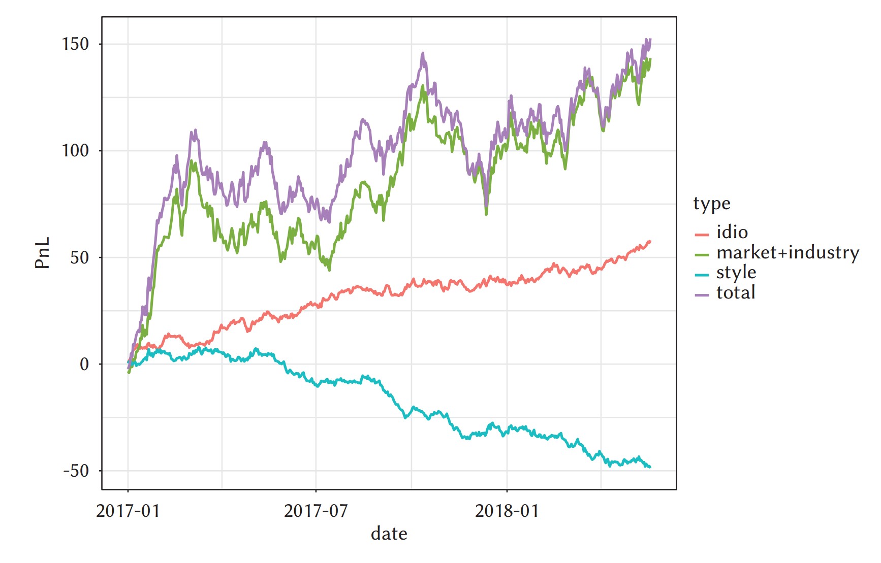
The figure shows the cumulative PnL (Profit and Loss) over time for a portfolio with the following configuration:

• Portfolio structure: A US equity portfolio consisting of 400 long positions and 100 short positions — a typical net-long strategy.

• PnL Components:

  • Total PnL (purple line): The full observed PnL of the strategy.
  • Idiosyncratic PnL (red line): Gains/losses not explained by any known factor — stock-specific performance.
  • Market + Industry PnL (green line): Performance attributable to broad market movements and sector-specific trends.
  • Style PnL (blue line): Performance due to style factors like value, momentum, size, etc.

Key Observations

• Total PnL and Market + Industry PnL Track Closely:

  • The purple and green lines closely follow each other throughout the time horizon.
  • This implies that most of the total portfolio performance is due to market and industry exposure — not necessarily manager skill.
  • The high Sharpe Ratio of 1.56 is impressive on the surface, but likely reflects favorable beta exposure rather than true alpha.

• Idiosyncratic PnL Adds Steadily but Modestly:

  • The red line shows slow but consistent gains.
  • This suggests the PM is capturing some stock-picking skill, but it is not the dominant driver of returns.

• Style PnL Is Negative:

  • The blue line trends downward sharply, indicating that exposure to style factors (e.g., value, growth, momentum) was detrimental over this period.
  • The PM may have had unintended or poorly performing style tilts — perhaps being overweight value in a growth-driven market, for example.

---

• Sharpe Ratio Misleading Without Decomposition:

  • A Sharpe Ratio of 1.56 could be interpreted as skill, but this figure alone obscures the contributions of systematic factors.
  • Most strategies report beta and benchmark-relative returns, but few show time-series PnL attribution as in this chart — which gives a more truthful picture.

• Net of Market + Industry Isn’t Enough:

  • If one only looks at total PnL minus market and industry (i.e., looking at style + idio PnL), one might still miss that some style exposures consistently detract from performance.
  • A full attribution like this one highlights potential weaknesses in portfolio construction (e.g., unwanted style exposure) that are not visible in basic relative performance metrics.

---

Example 2:

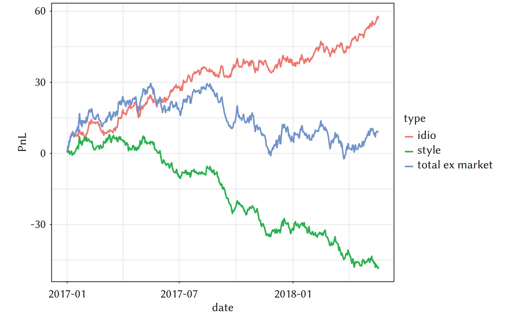
Total ex Market PnL (blue line):

• This line shows total portfolio PnL excluding market return (i.e., net of market exposure).
• It performs moderately — flat to slightly positive in early months, but mostly stagnating or declining after mid-2017.
• This mediocrity signals that without the market’s help, the portfolio’s core alpha is unimpressive at first glance — which raises questions about true skill.

🔴 Idiosyncratic PnL (red line):

• The real highlight: this component steadily rises, showing consistent outperformance from stock-specific bets.
• It achieves a Sharpe Ratio of 2.4, an exceptional result indicating that the PM has strong stock selection skill.
• This suggests that the manager does have alpha, just hidden beneath noisy factor exposures.

🟢 Style PnL (green line):

• Style factor exposure (value, momentum, size, etc.) has consistently detracted from performance.
• It not only fails to contribute but largely cancels out the positive idiosyncratic gains.
• This drag from style factors offsets the manager’s true edge.

Why This Is Actually Good News:

• Unlike market exposure (which the manager may not fully control), style risk is manageable.

• The underperformance isn’t due to lack of skill — it’s due to factor misalignment, which can be quantified, monitored, and hedged.

• With proper factor risk management, the portfolio could unlock the full benefit of its stock-picking ability.

• Recurring Theme:

  • A core argument in the book is that factor PnL is not destiny — it can and should be actively managed.
  • This chart motivates going one level deeper in decomposition, likely into individual factor-level attribution (e.g., Value, Momentum, Low Vol).

---

Example 3:

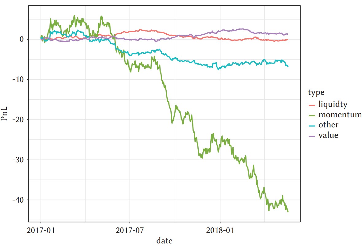
In this chart, we examine the component-level drivers of style factor performance for the portfolio over the 2017–2018 period. Specifically, we decompose the Style PnL (which was shown to be negative in Figure 8.2) into its individual factor contributions:

• Momentum (green)
• Value (purple)
• Liquidity (red)
• Other (cyan)

Key Observations

🟢 Momentum PnL:

• The dominant negative contributor by far.
• Momentum PnL plummets over the entire period, especially after mid-2017, reaching around –40 units by early 2018.
• This clearly indicates that the portfolio had sustained positive exposure to momentum, during a period in which momentum performed poorly.
• The manager was effectively "long momentum" in a momentum drawdown.

🟣 Value PnL:

• Very stable and slightly positive — a neutral to mildly helpful factor.
• This tells us value exposure was not significantly influencing the portfolio outcome during this time.

🔴 Liquidity PnL:

• Also flat and neutral — no meaningful impact on the portfolio’s performance.

🔵 Other Style PnL:

• Slightly negative, but its scale is small compared to momentum.
• Likely includes secondary style dimensions (e.g., low volatility, size) that weren’t dominant contributors.

---

Supporting Evidence

• The average exposure to momentum was positive, meaning the portfolio systematically favored momentum stocks.
• Momentum explained a large portion of the portfolio’s factor risk, both in terms of exposure magnitude and variance contribution.

This aligns with the sharp and prolonged drawdown in the momentum line on the graph.

---

• The poor total ex-market performance (Figure 8.2) was not due to lack of alpha, but to a single unintended or unmanaged risk: momentum.
• The PM may have been unaware of this exposure or underestimated the impact of momentum on factor variance.
• Momentum exposure is not inherently bad — but like all factor tilts, it should be intentional and managed.
• This kind of breakdown is invaluable for risk-aware portfolio construction.

---

Core Idea: True investment skill lies in understanding and improving idiosyncratic performance—not just managing factor risk—which requires analyzing selection, sizing, timing, and diversification.

• Limitations of factor management:

  • Controlling factors protects performance but doesn't create profitability.
  • Factors can distort returns but don't generate alpha.

• Misconception about idiosyncratic returns:

  • Even though single-stock idiosyncratic PnLs are uncorrelated, this doesn't guarantee true insight or effectiveness.
  • Differences in risk levels per position complicate this picture.

• Key analytical areas:

  1. Sizing skill:

     • Evaluates whether returns match the risk-adjusted conviction in position sizes.

  2. Temporal behavior:

     • Portfolios are dynamic, not static snapshots.
     • Understanding how ideas evolve and decay over time is essential.

  3. Three-component decomposition:

     • Selection: Did you pick the right stocks?
     • Sizing: Did you bet the right amount?
     • Timing: Did you enter/exit at the right moment?
     • These reflect the core dimensions of investing style and edge.

  4. Diversification and hit rate:

     • Explores how portfolio breadth and success frequency interact, affecting overall strategy quality.

Core Idea: Decomposing idiosyncratic PnL into selection, sizing, and timing components provides a structured way to understand and improve the distinct dimensions of portfolio management skill.

• PnL decomposition framework:

  • Idiosyncratic PnL = Selection PnL + Sizing PnL + Timing PnL

    • Selection: Directional correctness in stock picking.
    • Sizing: Appropriateness of bet sizes relative to conviction.
    • Timing: Ability to take on risk at the most favorable times.

• Stock Selection & Sizing:

  • Rearranging historical data into a matrix enables "what-if" analyses (e.g., equal-sizing simulations).

  • Cross-sectional equalized (XSE) portfolios remove sizing effects to isolate selection skill.

  • Equal sizing tends to reduce volatility and improve Sharpe, even if absolute returns fall.

  • Insights from sizing analysis:

    • Identify strengths and weaknesses between long and short books.
    • Guide adjustments in position sizing to optimize returns and Sharpe ratios.
    • Be mindful of liquidity constraints, which can invalidate purely theoretical sizing models.

• Liquidity-adjusted analysis:

  • Incorporates trading volume constraints (e.g., max percentage of daily volume traded).
  • More realistic simulations reflect gradual position building/unwinding, especially in illiquid stocks.

• Timing Analysis:

  • Captures whether a PM can align exposure with periods of favorable returns.
  • Fundamental investors often lack timing skill due to their long-term, strategic focus.
  • Negative timing can be corrected via position and exposure equalization across time.

• Cross-sectional time-size equalized (XSTSE):

  • Normalizes position sizes both within each date and across time, eliminating timing and sizing effects.
  • Facilitates the pure measurement of selection skill.

• Practical outcomes:

  • Quantifying each component helps PMs identify their specific strengths and weaknesses.
  • If sizing or timing skill is lacking, defaulting to equal sizing/time-normalization can enhance performance.
  • Regular monitoring of these dimensions supports continuous improvement.

• Key insight:

  • Most PMs exhibit:

    • Strongest skill in selection.
    • Weak-to-moderate skill in sizing.
    • Generally poor or neutral timing skill.

  • Recognizing and leveraging even modest skill in any of these areas is valuable.

Core Idea: Diversification enhances risk-adjusted performance by amplifying even modest forecasting skill, but its benefits plateau if increasing breadth dilutes accuracy.

Improves Information Ratio (IR) via Diversification

• The Information Ratio (IR) measures risk-adjusted active return:

  $$ IR = \frac{\text{Expected Active Return}}{\text{Tracking Error (volatility of active return)}} $$

• This specific formula links IR to two key variables:

  $$ (\text{Inf. Ratio}) = \left[ 2 \times (\text{hitting probability}) - 1 \right] \times \frac{1}{\sqrt{252 \times (\text{effective number of stocks})}} $$

  • Hitting Probability: Probability that your position is correctly aligned with the asset’s idiosyncratic return.
  • Effective Number of Stocks: Adjusted count of positions accounting for concentration. If weights are uneven, the effective number is lower than the actual count.

• The square root relationship means:

  • To double your IR, you need 4x the effective number of independent stocks, assuming the same hitting probability.
  • Simply adding more names doesn’t help if they're highly correlated or if positions are overly concentrated.

---

🔍 Effective Number of Stocks

• It's a measure of diversification beyond naive stock count.

• Formulaically, sometimes approximated as:

  $$ \text{Effective Number} = \frac{1}{\sum w_i^2} $$

  where $w_i$ is the weight of each stock. This penalizes concentrated weights.

• Even if you hold 3000 stocks, if weights are heavily skewed to the top 100, your effective number might only be ~100-200.

---

🎯 Hitting Probability

• Definition: Probability that your position is aligned with the asset’s idiosyncratic return.

  • Long + positive return or short + negative return.

• Even a modest edge—like 51% accuracy—compounds with diversification.

🧩 Practical Examples

1. 51% hit rate with 70 effective stocks:

   $$ IR = (2 \times 0.51 - 1) \times \frac{1}{\sqrt{252 \times 70}} \approx 2.6 $$

2. 50.5% hit rate with 3000 effective stocks:

   $$ IR = (2 \times 0.505 - 1) \times \frac{1}{\sqrt{252 \times 3000}} \approx 8 $$

• This is why stat-arb and high-frequency strategies with marginal predictive signals (barely above 50%) can still achieve extraordinary risk-adjusted returns—because of:

  • Large numbers of independent bets
  • Controlled position sizing to maximize effective stock count.

---

✅ Key Takeaways

• Boosting hitting probability is valuable, but increasing the effective number of stocks is often more scalable.
• Diversification reduces the volatility of active returns, allowing small predictive edges to produce high IR.
• Effective number, not raw number, is critical: Concentration and correlation reduce its benefit.

---

• Critical limits:

  • Diversification is a "skill multiplier," not a skill itself.

  • Beyond a point, adding stocks can reduce accuracy (hitting probability drops) due to:

    • Time constraints.
    • Coordination overhead when teams expand.

  • There's an optimal breadth where the marginal benefit of added diversification equals its cost to accuracy.

• Real-world caution:

  • Year-to-year performance comparisons are noisy due to standard error in hit rate estimation (~0.33% annual standard error), making small gains hard to confirm.
  • Expanding coverage by hiring analysts with similar hit rates is preferable to spreading PM attention thinner.

Core Idea: Alternative data presents a major opportunity for alpha generation and risk analysis, but its effective use requires structured, collaborative processes to evaluate, transform, and integrate such data into fundamental investing.

• Significance of alternative data:

  • A defining trend in finance, akin to "new oil"—abundant, valuable if properly processed.
  • Includes transactional data, satellite imagery, unstructured text/images, etc.
  • Initially embraced by quants, now increasingly used by fundamental investors.

• Key challenges for PMs:

  1. Purpose clarity: Define whether data aids alpha generation, risk prediction, or tail risk assessment.
  2. Visualization: Determine how to summarize and present the data effectively.
  3. Value assessment: Develop tests to assess predictive power beyond hindsight claims.
  4. Integration: Align data insights with the fundamental investment process.

• Practical framework for using alternative data:

  • Leverage factor model structures for incorporation:

    • Compress data into single-stock characteristics (akin to factor loadings).
    • Evaluate if characteristics predict residual (unexplained) returns.
    • Incorporate only if predictive power is sufficiently high.

• Data scientist + investment analyst collaboration:

  • Data scientists: Handle technological and statistical processing.
  • Analysts: Provide domain knowledge, guide relevance, and contextual interpretation.

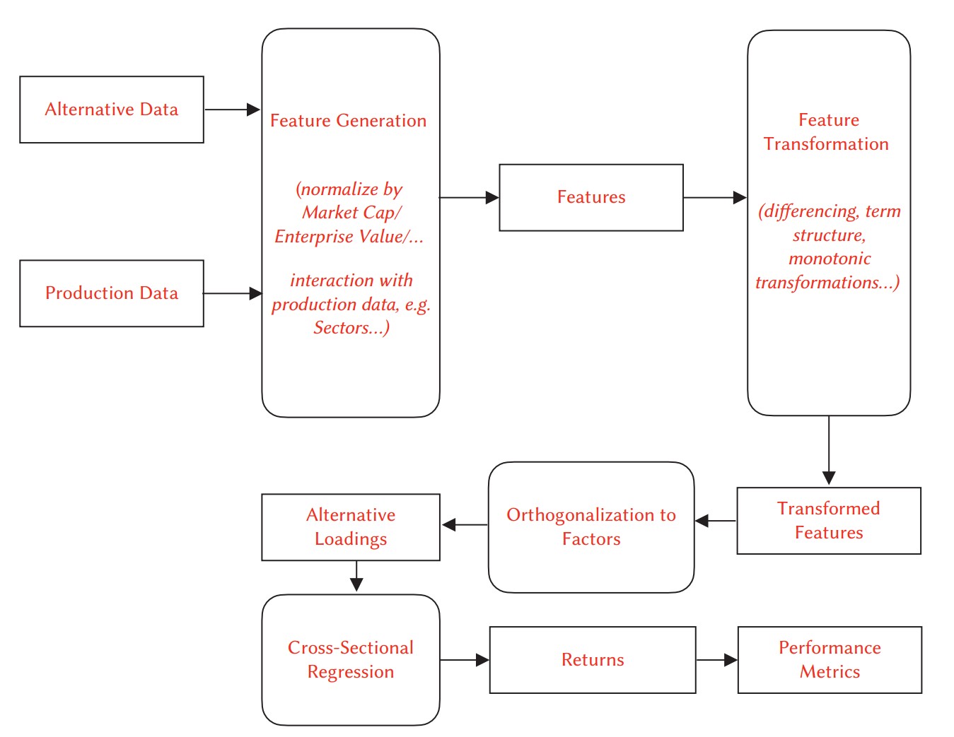
• Processing steps (illustrated via Short Interest data example):

  1. Feature generation: Derive raw features (e.g., borrow rate, short ratio).
  2. Feature transformation: Normalize or compare features to historical baselines.
  3. Orthogonalization: Remove overlaps with existing risk model factors.
  4. Cross-sectional regression: Test correlation with asset returns.
  5. Performance evaluation: Check for persistent, non-zero expected returns, Sharpe ratios, and stability.

• Strategic caution:

  • Avoid data mining and overfitting by limiting arbitrary feature creation.
  • Focus on data that's sector, industry, or geography relevant.
  • Cross-sectional analysis preferred over complex time-series forecasts, given the difficulty of timing.

• Broader vision:

  • Although full "data in, strategy out" automation remains aspirational, integrating alternative data incrementally through structured, empirical methods enhances both alpha discovery and risk control.

Core Idea: Common discrepancies and uncertainties in performance attribution arise from methodological limits, multiple contributing factors, and the inherent variability in Sharpe ratio assessments—requiring both domain judgment and quantitative rigor.

• Attribution vs. OMS/Treasury reports:

  • Attribution uses end-of-day data, missing intraday trading PnL.
  • Currency effects can create mismatches if not fully hedged or itemized.

• Idiosyncratic PnL confusion:

  • A stock can show negative idio PnL despite gains if broader market, sector, or style factors contribute more than the stock's return.
  • Understanding factor contributions clarifies discrepancies.

• Sharpe ratio sensitivity:

  • Changes in Sharpe from "what-if" analyses may or may not be significant:

    • If testing a specific, informed hypothesis, small improvements can be meaningful.
    • In exploratory (data-mined) tests, caution is warranted.

  • Quantitative methods can adjust Sharpe for multiple testing biases ("Sharpe haircut").

    • Formal methods are available via academic research (e.g., Harvey et al. 2016).

• Best practice:

  • Combine domain expertise for hypothesis-driven tests with quantitative analysis for validation and statistical adjustments.