Design, test, optimization and evaluation of a trading system

Designing a Trading System

Innovation and Idea Generation

• Creativity and Inspiration:

  • Innovation lies between creativity and fancy.
  • Good trading system ideas often come unexpectedly.
  • Engaging with experienced traders and attending seminars, congresses, and meetings can spark new ideas.
  • Observing discretionary traders at work can also provide inspiration.

• Getting Started:

  • Internet Resources:
    • Search for terms like “trading systems” and “AmiBroker” for videos and code examples.
  • Literature:
    • Review existing books on algorithmic trading.
    • Use the bibliography of relevant books as a starting point.
  • Forums:
    • MultiCharts, TradeStation, and AmiBroker forums offer free trading codes and ideas.

The Programming Task

• System Components:

  • Entry Formula: Defines when to enter a trade.
  • Exit Formula (Risk Management):
    • Manages how much money is risked in each trade.
    • Includes initial stop loss, trailing stop, and target exit.
  • Money Management Formula:
    • Determines how much to invest in each trade.
    • Decides the number of stocks or futures contracts to buy or sell.

• Importance of Money and Risk Management:

  • Effective money management and risk management tools are crucial for making a trading system viable.
  • Extensive use of leverage and money management techniques can lead to astonishing returns, but must be applied appropriately.

Which Timeframe to Trade?

Intraday vs. Daily Trading

• Retail vs. Institutional Preferences:

  • Retail Traders: Often prefer intraday trading, perceiving it as lower risk.
  • Institutional Traders: Typically avoid the effort of 24-hour market monitoring required for intraday trading.

• Globalization and 24-Hour Markets:

  • Most futures contracts are traded 24/7 on platforms like Globex.
  • Major price moves still occur during US daylight sessions, but globalization has made markets active around the clock.
  • Liquidity now moves seamlessly across global markets, enabling traders to participate in foreign markets (e.g., US traders trading German DAX futures).

• Future Market Trends:

  • Anticipated that there will be little difference between trading during the day or night as markets become continuously active.

Intraday Trading

• Pros and Cons:

  • Pros:
    • Potential for quick gains due to frequent trading opportunities.
  • Cons:
    • Highly demanding and requires constant monitoring.
    • Not compatible with other work unless shared among a team.
    • Exposure to sudden price movements, energy blackouts, and platform inefficiencies.

• Recommendation:

  • Best suited for teams of at least three traders to share the burden of 24-hour monitoring.
  • Essential to have multiple strategies to mitigate risks.

Daily Timeframe Trading

• Pros and Cons:

  • Pros:
    • More relaxed approach, suitable for traders with other occupations.
    • Easier to manage with disciplined daily order placements and position checks.
    • Reduced exposure to sudden market shocks compared to intraday trading.
  • Cons:
    • Larger drawdowns in absolute monetary terms.
    • Longer periods of flat equity lines.

• Risk Management:

  • Choose futures contracts with appropriate margins, volatility, and liquidity to level out drawdown and risk.

Importance of Market Data in Testing Trading Systems

Data Accuracy and Trustworthiness

• Challenges with Market Data:

  • Access to market data is now cheap and easy.
  • Despite accessibility, verifying the trustworthiness of data is crucial.
  • Data discrepancies can affect trading algorithm outcomes.

• Common Data Vendor Issues:

  • Different interpretations of closing prices vs. last traded prices.
  • Variations in open prices, especially from auction-based openings.
  • Inconsistent daily high and low prices.
  • Confusion during irregular trading sessions (e.g., CME futures on Sundays).

• Ensuring Data Accuracy:

  • Compare data series from multiple vendors.
  • Recommended data sources for commodities and futures:
    • CSI Data
    • Pinnacle Data
    • TradeStation
    • Norgate Data

Long-Term Stock Data Challenges

• Stock Price Series Issues:

  • Corporate actions (mergers, splits, bankruptcies) impact long-term accuracy.
  • Example: Vodafone's acquisition of Mannesmann, Dow Chemical and DuPont merger.

• Dividend Adjustments:

  • Price series must be adjusted for dividend payments.
  • Ensure use of high-quality data suppliers like Norgate Data.

Futures Price Series Challenges

• Expiration Dates:

  • Futures have varying durations (e.g., 1 month for NYMEX Crude Oil, 14 months for cereal futures).
  • Connecting expiration dates over long periods is complex.

• Methods to Connect Futures Contracts:

  1. Same Expiration Contracts:
     • Connect contracts of the same expiration month across different years (e.g., September Corn 2001, 2002, 2003).
     • Suitable for commodities with seasonal patterns (e.g., US corn).
  2. Continuous Contracts:
     • Collage of different forthcoming delivery months.
     • Most liquid and traded contracts form the price series.
     • Price gaps occur on delivery days, reflecting real trading conditions.
  3. Perpetual Contracts:
     • Avoids delivery day price gaps.
     • Mathematical representation where old prices are updated based on the last expiration day's gap.
     • Point-based or ratio-adjusted updates keep relative historical price swings constant.
     • More complex methods exist

The Length of Your Back-Testing Period

Importance of Multi-Period and Multi-Market Testing

• Multi-Period Testing:

  • Ensures a trading system's robustness and consistency over time.
  • Markets continuously evolve due to changes in the economy, institutions, and society.
  • Some traders test intraday systems for only 3 to 12 months, while others advocate for longer periods.

• Multi-Market Testing:

  • Tests the system's effectiveness across different types of markets (bonds, equities, commodities, currencies, stocks).
  • Systems usually perform well in specific markets rather than universally across all markets.

Practical Considerations for Back-Testing

• Historical Context:

  • Avoid testing on data from periods with significant structural changes or anomalies.
  • Example: Testing on a banking stock before and after a major merger.
  • Example: Using euro/dollar data derived from Deutsche mark/dollar before 2003.

• Exclude Abnormal Periods:

  • Exclude data from periods of extreme market conditions, such as the stock bubble (1999–2000) or the crude oil spike (2008).
  • Focus on normal market conditions, which constitute approximately 80% of the time.

Guidelines for Choosing the Back-Testing Period

• Ordinary Acumen:

  • Use experience and practical judgment to decide the appropriate back-testing period.
  • Consider the nature of the asset and significant historical events that may affect price behavior.

• Avoiding Overfitting:

  • Ensure the system's parameters are not overly tailored to specific historical data.
  • Balance between testing period length and data relevance to current market conditions.

Rule Complexity and Degrees of Freedom in Trading Systems

Purpose of Multi-Market Testing

• Primary Aim:

  • Verify if a system performs as intended across different markets.
  • Ensure the system is profitable on average, even if not in every market.

• Importance of Testing:

  • Validates the statistical soundness of the system.
  • Optimisation: Fine-tunes the system for specific market behaviors after initial testing.

• Expected Outcomes:

  • Systems typically perform well in similar markets (e.g., all energy futures) but may perform differently in diverse markets (e.g., bonds vs. currencies).

Deciding the Test Window Size

• Statistical Requirements:
  • Length: The price series must cover various market situations and generate a significant number of trades.
  • Degrees of Freedom: The number of variables and conditions should not exceed 10% of the total data sample.

Understanding Degrees of Freedom

• Definition:

  • General: The number of independent components minus the number of estimated parameters.
  • Simplified Example: In a regression, with one data point, you can't estimate a regression line (degrees of freedom = 0). With two points, you can (degrees of freedom = 1).

• Importance:

  • The wider the sample size and the fewer the variables, the better the estimation accuracy.

• Practical Calculation:

  • Formula: Degrees of freedom = total data sample - (rules and conditions + data consumed by rules and conditions).
  • Aim to retain at least 90% degrees of freedom after accounting for system variables.

Example Calculation

• Scenario:
  • Data Sample: 3 years of daily highs, lows, opens, and closes = 3120 data points.
  • Trading Strategy: Uses a 20-day average of highs (21 degrees of freedom) and a 60-day average of lows (61 degrees of freedom).
  • Calculation: Total degrees of freedom used = 82. Remaining degrees of freedom = 97.4%.

Number of Trades for Reliability

• Significance of Trade Count:

  • The system must produce enough trades to minimize the risk of random success.
  • Rule of Thumb: At least 100 trades are needed for a trustworthy system.

• Standard Error Calculation:

  • Formula: Standard Error = $\sqrt n + 1$, where n = number of the trades
  • For 100 trades, the standard error is ±10%.

The Forecasting Power of a Trading System

Optimisation

• Definition and Purpose:

  • Optimisation: Adjusting system variables to maximize profits or meet specific constraints (e.g., minimizing drawdown).
  • Example: Determining the optimal number of days for short-term and long-term moving averages in a crossover system.
  • Goal: Adapt the system to the market it trades in terms of volatility, risk, return, etc.

• Pitfalls of Optimisation:

  • Over-Optimisation (Curve Fitting):
    • Finding inputs that made the most money in the past but lack forecasting power.
    • Example of Poor Optimisation: A system that buys at the lowest price and sells at the highest price daily, which is unrealistic.

• Inevitable Optimisation:

  • All traders engage in some form of optimisation, whether consciously or not.
  • Examples of Involuntary Optimisation:
    • Choosing a system based on past performance.
    • Modifying system code to fit market behavior and selecting the best historical variation.

• Distinguishing Useful Optimisation from Over-Optimisation:

  • Normal Optimisation:
    • Fine-tunes the system to market characteristics within a reasonable timeframe.
    • Ensures the system remains relevant to current market conditions.
  • Over-Optimisation:
    • Adjusts the system excessively to past data, losing forecasting power.

Practical Approach to Optimisation

• Monetary Policy Example:

  • Context: Trading a daily system on bond futures influenced by monetary policy.
  • Optimisation Window: 6, 12, or 18 months to align with economic cycles.

• Testing and Fine-Tuning:

  • Initial Testing: Use the longest available price series to check if the system can capture market moves.
  • Regular Re-Optimisation: Re-optimize the system every 6 to 12 months to keep it aligned with market changes.

• Evaluation:

  • The equity line should show growth, even if not perfectly smooth.
  • Initial Testing: Determines if the system is suitable for the market.
  • Optimisation: Identifies potential improvements through input changes.
  • Re-Optimisation: Periodically adjusts the system to maintain its effectiveness.

• Intraday Systems:

  • Shorter testing, optimisation, and re-optimisation periods compared to daily or weekly systems.

Walk-Forward Analysis

Evolution of Optimisation

• Traditional Optimisation:

  • Included an "out-of-sample period" (usually 10–20% of the optimisation window) to verify forecasting power over unseen data.
  • If the system performs well on the out-of-sample data, it indicates robustness.

• Modern Optimisation:

  • Evolved into walk-forward analysis (WFA), a more efficient and proper method for testing systems over long price series.

Walk-Forward Analysis (WFA)

• Methodology:

  • Rolling Walk-Forward Analysis:
    • Optimise the system over an initial period (e.g., 2 years).
    • Apply it to the subsequent 6 months of unseen data.
    • Move the optimisation window forward by 6 months and repeat the process.
  • Anchored Walk-Forward Analysis:
    • Start period remains the same.
    • Optimisation period extends as time progresses.
  • Application:
    • Rolling walk-forward analysis is more appropriate for intraday systems due to changing market conditions.

• Realistic Equity Line:

  • The equity line from a walk-forward run reflects real trading conditions more accurately.
  • Different from the equity line produced by testing and optimising a trading system on the entire price series.

Measuring Forecasting Power

• Walk-Forward Efficiency Ratio:
  • Ratio between the annualised net profit from walk-forward tests and the annualised net profit from optimisation periods.
  • Efficiency Threshold:
    • Above 100%: High probability of retaining forecasting power during real trading.
    • 50%: Minimum acceptable level, indicating the system performs at least half as well as during optimisation.
  • Importance of Multiple Tests:
    • Perform at least ten walk-forward analysis tests.
    • Ensure the test window covers at least 10–20% of the whole optimisation price series.

Practical Tips for Optimisation

• Ordinary Optimisation Process:

  • Before using WFA, perform basic optimisation to understand the system's performance.
  • Use shift tests to quickly check system robustness.

• Optimising Multiple Inputs:

  • Test one or two inputs at a time while keeping others static.
  • Minimizes the risk of over-optimisation by avoiding simultaneous optimisation of all inputs.

Key Takeaways

• Modern Optimisation with WFA:

  • Provides a realistic assessment of a trading system's performance.
  • Reflects actual trading conditions better than traditional optimisation methods.

• Efficiency and Robustness:

  • Use the walk-forward efficiency ratio to gauge system robustness.
  • Aim for ratios above 100% for high confidence in system performance.

• Optimisation Best Practices:

  • Perform initial optimisation and shift tests to understand the system.
  • Optimise inputs sequentially to avoid over-optimisation.

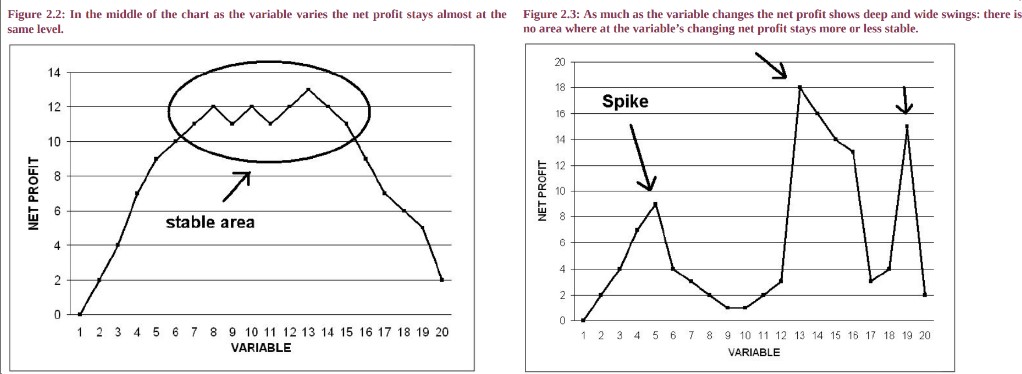
Robustness But can we deduce from the post-optimisation window if the system is robust or whether it is the product of over-optimisation? We do not need to trust the area of the best performing inputs as a sure way to victory. If enough darts are thrown at the board, a high-scoring grouping will occur or, put in another manner, if a monkey is put in front of a piano and enough time is allotted, it will eventually compose a sonata. This joke suggests that, at least, the average of the results should be profitable if we want to trust the most performing inputs. If just 1% to 5% of the results are profitable this could have happened by accident: if the system’s variables are given wide enough input ranges eventually the system will make a fortune over the past data. A robust system will show post-optimisation positive performances not only in 5% of all the tests but on the average of the tests. In other words, if the average results are positive then we can assume that the trading system is a robust one. If you are more statistically inclined you can also subtract the standard deviation (or a multiple of it) from the average net profit and check if the average net profit remains positive in this case. So the number of inputs, conditions and variables must be kept under control and reduced to its minimum term. But how many inputs, conditions and variables are too many? This is a controversial area where the unique hallmark is the number of degrees of freedom that must always respect the numerical condition we depicted in the previous paragraph. Before taking an input into consideration it is obviously important to check with a rapid and cursory optimisation if the input varies or if it does not have any change under optimisation. If not, keep it constant in order to increase the degrees of freedom. Another point to be considered is what scan range to choose for each input. An example will give a clearer picture of this problem: if you want to test a moving average crossover system with a short-term moving average and a long-term moving average on daily data, you cannot test the short moving average from 1 to 20 (this is what is considered the short term with daily data) and the long moving average from 20 to 200 (the latter is the interval that is usually considered long term with daily data). Indeed a step from 1 to 2 is a 100% change and a step from 19 to 20 is a 5% change. But a step change from 199 to 200 is just a 0.5 % change. You need to put the step scan range in an almost parallel relationship so that the scan from 1 to 20 will be performed with a step of 2 and the scan from 20 to 200 will be performed with a step of 20. After optimisation is done a critical decision should be taken: which inputs’ batch should we choose? First of all what we need to do is create a function chart that puts the variable’s inputs scan range in relation to the net profits (or whichever other criteria was chosen for optimisation) What we are looking for is a line that ideally would be as close as possible to a horizontal line, so that the net profit is not dependent on the input values. Reality is much different from theory so that we should be content with a line that grows lightly, then tops for a while and then decreases. The topping level is what we are looking for, that is an area where, even when changing the inputs, the net profits stay almost constant. This is the area where the robust input values are. This is diametrically opposite to a profit spike, that is a point in the line where net profit is high but it decreases deeply in the surrounding values. In other words we need to find an area where even after changing the input values net profit stays stable. In summary we can state that there should be a logical path into the inputs’ results so that something coherent in terms of inputs’ batch should arise. When there is not a linear relationship with inputs and net profits, or drawdown, or whichever constraint you are putting as a primary rule of the optimisation, the whole set of results must be regarded as suspicious.